
From 2D to Depth
A log is 2D, a simple piece of text, sometimes slightly enriched. While we spend most of our time reading ugly log lines in our terminals, our SIEMs and other tools, attackers keep advancing faster and faster… To help us in this hunt for the bad guys, here’s a short blog post on graph-based representation of our data.
Fair warning: this is an essay meant to spark new ideas and new ways of working. It’s the first article in a series where I’ll present concrete examples of the concepts laid out here. I hope you enjoy it!
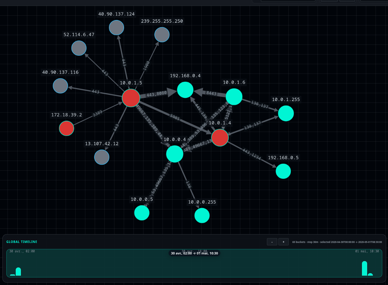
Result obtained from Zeek logs
What’s a Graph, Anyway
A graph is a data structure made up of nodes and edges that connect them.
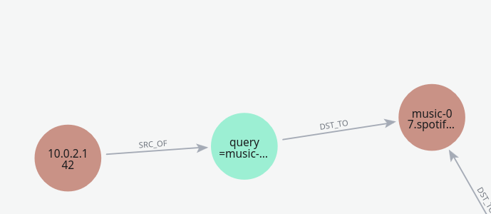
Example of a small graph representing a DNS query
Graphs are extremely useful for a wide range of problems in computer science: mapping, video games, social networks, etc. Anything that needs to be represented through relationships can be modelled as a graph.
A few useful definitions for the rest of this article:
- Directed relationship: a relationship with a direction. Example:
USER_A -> ADMIN_TO -> SERVER_01. - Undirected relationship: a relationship with no particular direction. Example: two machines connected to the same network.
- Property: a piece of information attached to a node or a relationship. Example:
name,ip,timestamp,port,protocol. - Path: a sequence of nodes and relationships that allows moving from point A to point B.
- Neighbour: a node directly connected to another.
- Degree: the number of relationships connected to a node. A node with many relationships is often called a hub.
To learn more about how graphs work, I’ll point you to this introduction from GeeksforGeeks.
Solving Problems with Graphs
Beyond providing a practical way to represent data, graphs bring a new approach to solving certain problems. For example, finding the shortest paths using Dijkstra’s algorithm or A*:
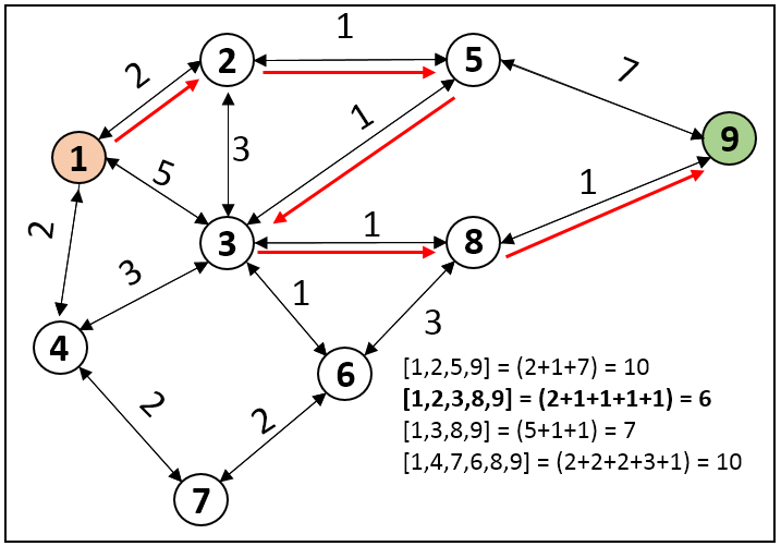
Example of shortest path resolution with Dijkstra’s algorithm
Several well-known databases exist for storing data in graph format; they implement an efficient storage mechanism for these objects and offer pre-implemented algorithms to ease their use. Among these databases, the notable ones include:
- ArangoDB: graphs + documents, very versatile.
- Neo4j: the graph reference, used by tools like BloodHound.
- JanusGraph: distributed graph, designed for large volumes and backends such as Cassandra/HBase.
These databases implement an efficient way of searching through relationships, something that databases like PostgreSQL or MongoDB simply don’t allow. They also offer pre-implemented graph algorithms, to make searching within databases easier.
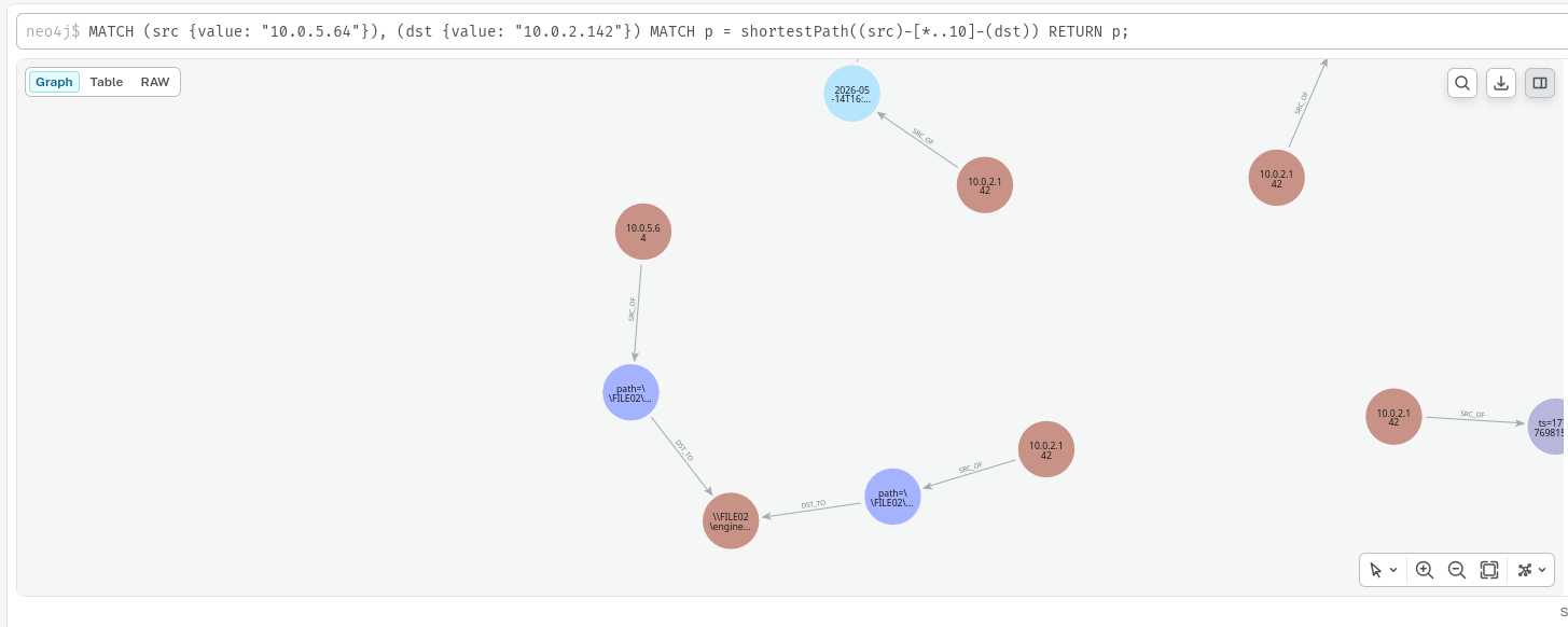
Demonstration of Neo4j’s shortestPath function
Worth mentioning too are the PageRank algorithms, which automatically identify the most important nodes in our graph. Originally designed to index web pages, they allow us to identify the central and critical nodes in a graph. Equally, this algorithm can be used to spot nodes that are barely referenced and potentially detect anomalies.
Graphs in Cyber
In cyber, every element is relational and a node can represent pretty much anything: a machine, a user, an IP address, a Kerberos ticket, a process… And an edge represents a relationship between two of these elements: a network connection, an authentication, a process execution, a file access.
Take a user account, for instance: it has rights, meaning relationships with other objects, and it also belongs to groups. That same account can be connected to certain machines, and other groups may have rights over it. All of these relationships can be represented as a graph.
What makes graphs particularly powerful is that they allow reasoning about paths. Not just what an element is, but how you can move from one to another and that’s precisely what we need to model an attacker’s movement through an information system.
There are several types of graphs, but the ones we’ll care about most are directed and weighted graphs. Each edge has a direction (an arrow) and carries a weight (a value).
Let’s see how to apply this structure to the attacker’s perspective.
The Graph from the Attacker’s Side
While we defenders think in terms of attack surface, network topology and vulnerabilities, an attacker thinks in graphs (even if they don’t know it).
For them, one step might lead to a second or a third, all the way to reaching their final objective.
Let’s take a group engaging in cybercrime, right at the very beginning of their attack. Each node represents an action that could be carried out by BG (i.e. Big Bad).
A Phishing Example
The nodes in red represent the steps already completed by the attacker.
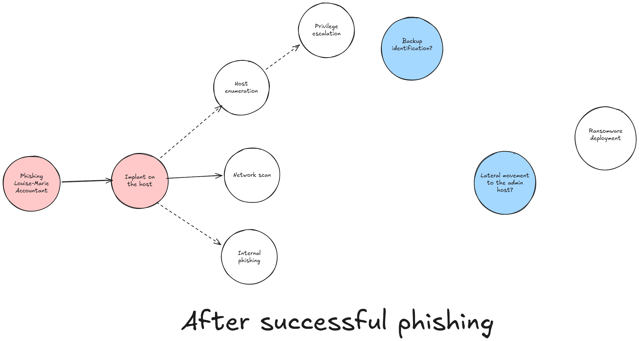
Above, BG (Big Bad) has just compromised the workstation of Louise-Marie, an accountant at a software development company.
Some of these steps will probably fail, and others will reveal new possibilities as they go.
If BG decides to push forward a little by performing a network scan of their surroundings, the progression might look something like this:
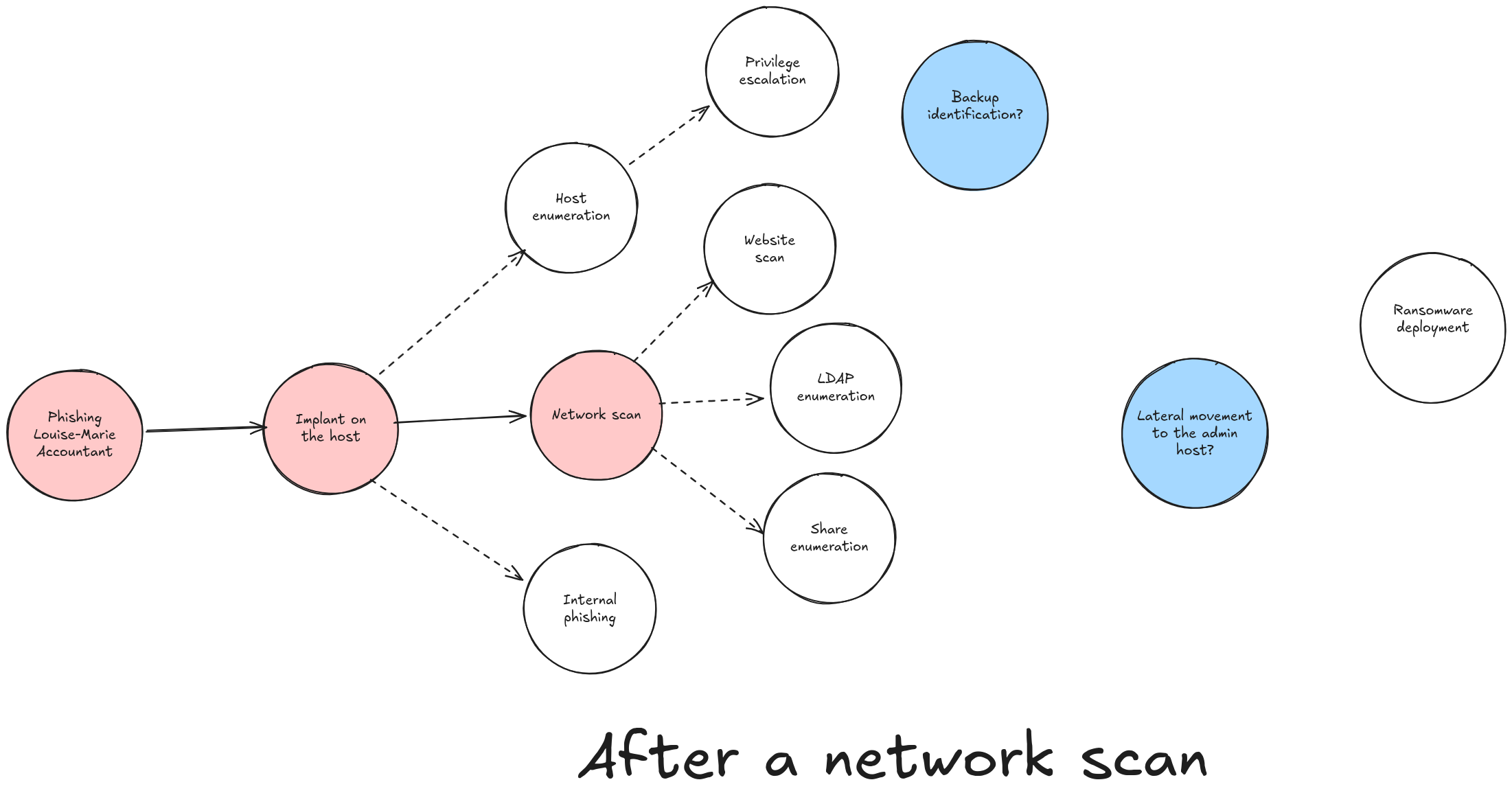
By performing a network scan, BG opens up new possibilities that will lead them, more or less quickly, to deploying their ransomware.
The BloodHound Example
BloodHound is the perfect example of graph thinking applied to offensive work. The tool is designed to find the shortest paths in a Windows environment towards a target objective.
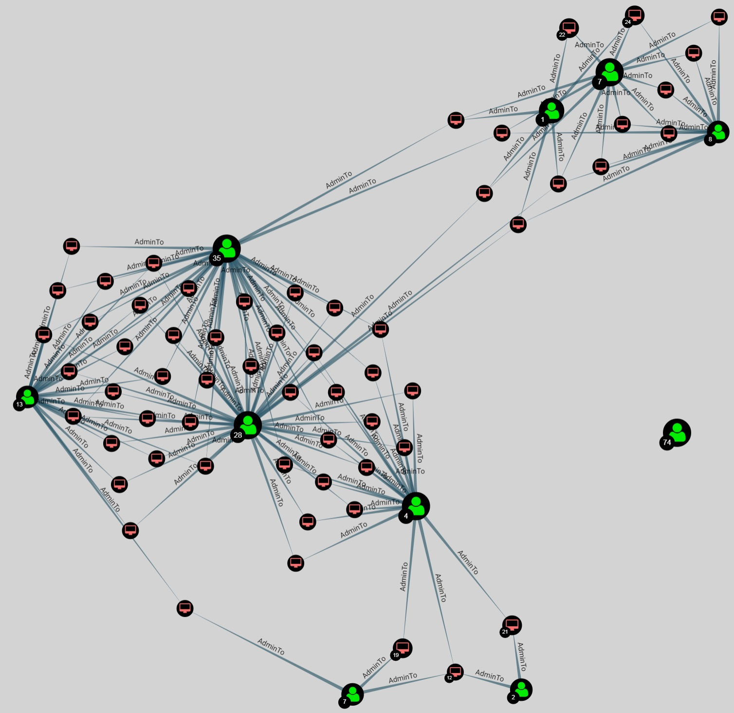
Here, shortest path search applies extremely well.
BloodHound graph representation
The Defender’s Graph Thinking
As Microsoft laid out in this article, a system to defend can be modelled as a graph. Being able to model an attacker’s possible progression through their network in graph form is interesting on several levels:
- identifying sensitive points to strengthen;
- setting up monitoring at strategic locations;
- running graph-based threat-hunting campaigns;
- understanding and containing the attacker during an incident response.
Imagine a graph capable of representing all the feared actions in our information system and the transitions between them:
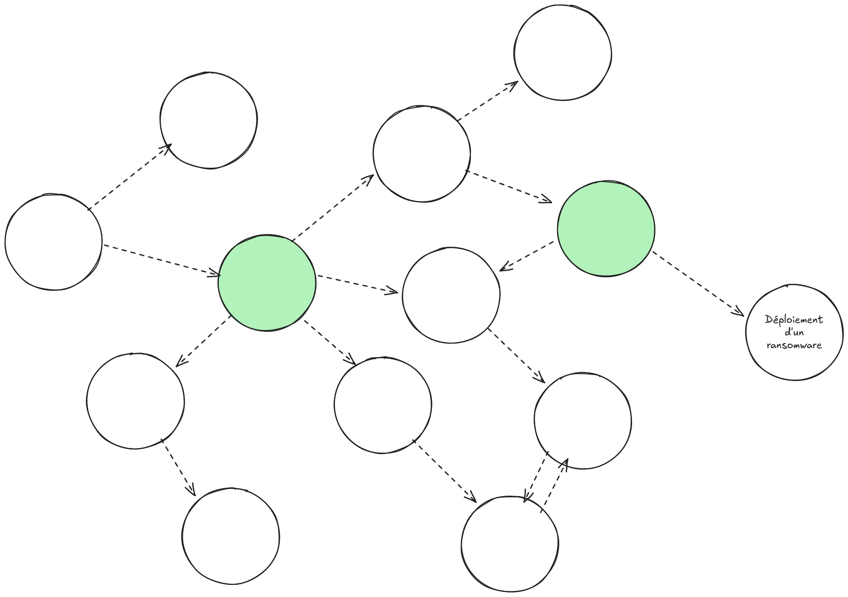
In the graph imagined above, two bottlenecks have been identified in green. These will be particular areas of focus in our information system where we can redouble our vigilance on monitoring and security.
Application to Digital Forensics
In DFIR, it’s often about starting from a cyber incident and pivoting through all the data at our disposal to find where the attacker may have gone and what they may have done.
What we call a pivot is nothing more than exploring the relationships of an event. By exploring its neighbours, we look for context, understanding, and sometimes even identify other malicious actions.
Here’s an example of a pivot on a TLS event:
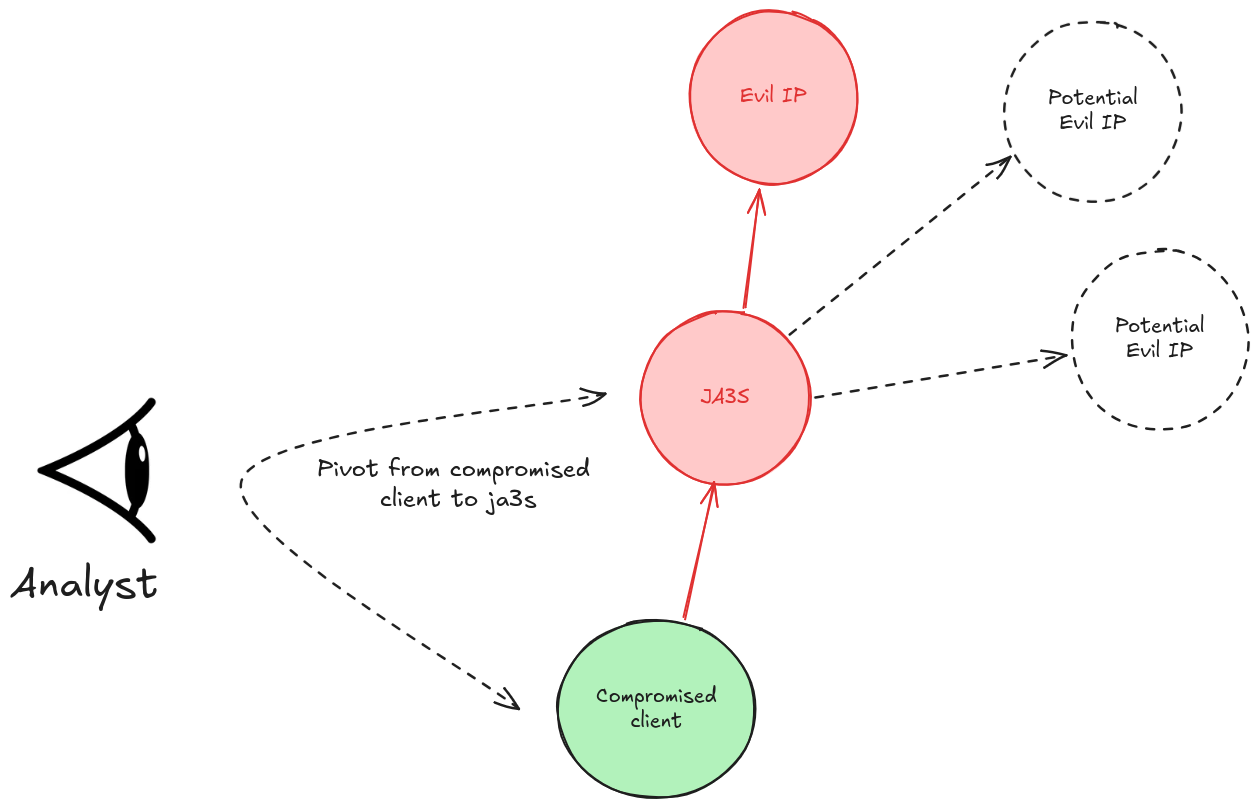
Above, during their investigation, the analyst identifies a new indicator: the JA3S fingerprint corresponding to the malicious server. By pivoting on this new indicator, they could identify new, previously unknown malicious servers.
In a Classic SIEM
To demonstrate what we’re talking about, we’ll use Zeek logs, an open-source solution that extracts useful data from the network, see my article on investigation with Zeek.
In ELK, it would look something like this:
Step 1 - we run our search on the compromised client:
FROM logs-zeek.ssl-*
| WHERE destination.ip == "24.234.1.1"
| KEEP source.ip, destination.ip, tls.server.ja3s, @timestamp
| SORT @timestamp DESC
We retrieve the JA3S: d41d8cd98f00b204e9800998ecf8427e. We pivot.
Step 2 - We look for all IPs that share this TLS fingerprint, excluding our already-known C2:
FROM logs-zeek.ssl-*
| WHERE tls.server.ja3s == "d41d8cd98f00b204e9800998ecf8427e"
    AND destination.ip != "24.234.1.1"
| STATS connexions = COUNT(*),
        premiers_contacts = MIN(@timestamp),
        sources = VALUES(source.ip)
    BY destination.ip
| SORT connexions DESC
In a Graph Tool
And here’s what a pivot would look like in a graph tool:
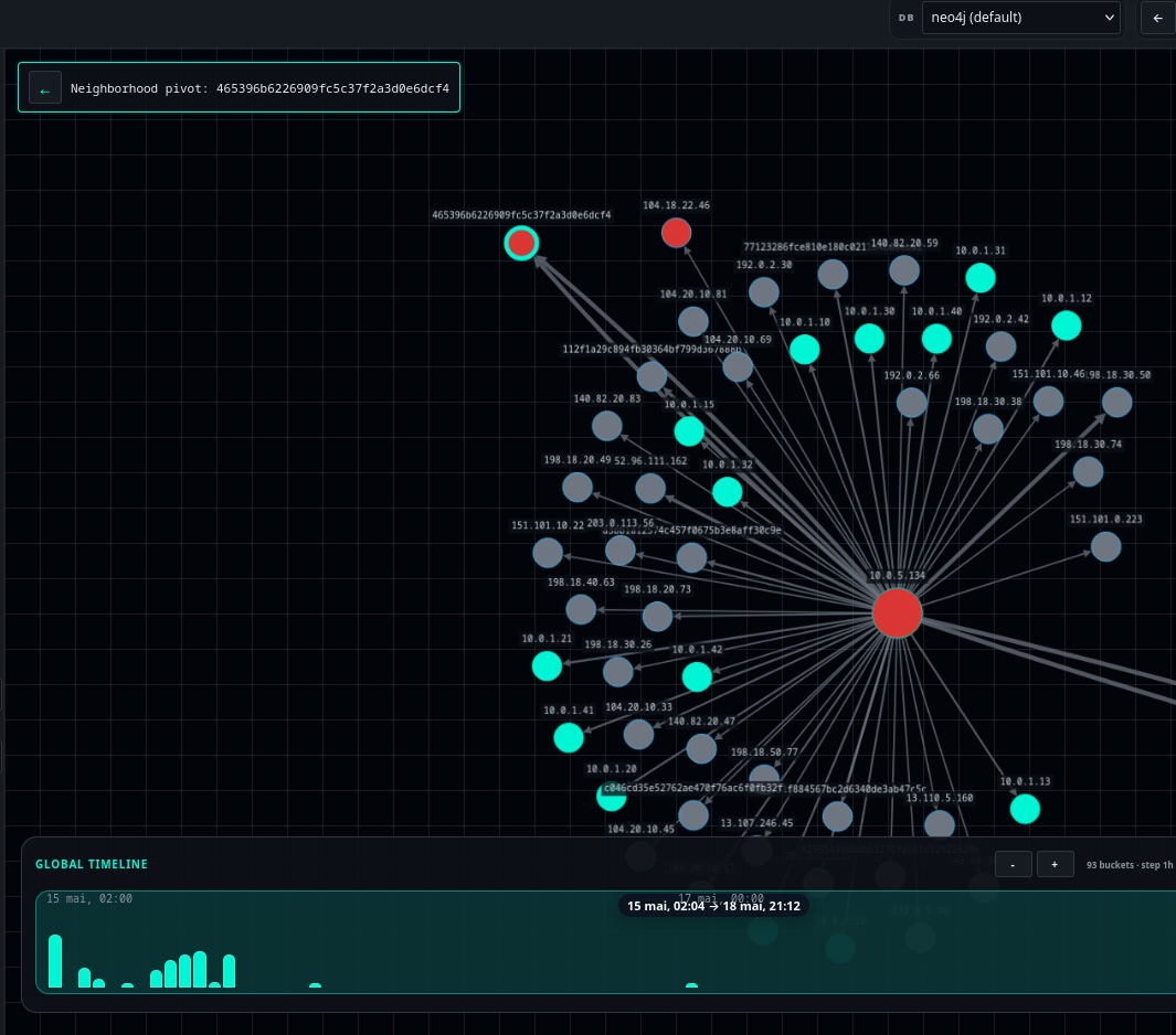
Here, a pivot on the JA3 465396b6226909fc5c37f2a3d0e6dcf4 would be performed with a simple right-click by the analyst. Colouring nodes identified as suspicious could also be done with another right-click.
All These Relationships
With the ability to expand all the relationships of a node, the analyst gains extraordinary speed. If we only considered Zeek logs, we could:
- pivot on all the neighbours of an IP;
- pivot on a domain name to identify who else is querying it;
- graphically link Kerberos tickets, the source IP and the destination service to identify anomalies;
- find the shortest paths between a compromised machine and servers to defend;
- trace all the relationships of a node at once to broaden our understanding of it.
All of this is quite difficult in a classic SIEM, but made much more obvious by working with graphs.
Towards Multidimensional Analysis
If we were able to feed all of our data into a graph database, we could greatly simplify analysis in a number of ways.
We’d move from two-dimensional logs to exploring, in a single click, all of their relationships.
Bridging CTI and Investigation Data
It’s often difficult to connect investigation data with OSINT data. Today, an analyst who stumbles upon a suspicious IP will open VirusTotal in one tab, Shodan in another, and manually cross-reference with their logs in a third. It’s laborious and it breaks the flow of the investigation.
If everything were represented in a single graph, with common observables as nodes IP, domain, hash, JA3S… pivoting between CTI and investigation data would become natural. You’d immediately see that an IP identified in your logs is also known from a threat intelligence report, and you could trace the thread in both directions without switching tools.
Anomaly Detection Through Machine Learning
Classic machine learning algorithms work on feature vectors: tables of values. But some suspicious patterns make no sense in a table, they only make sense in a relational structure.
An account bouncing from machine to machine outside its usual habits, a host starting to scan its neighbourhood, a process initiating connections that only another binary used to make… These behaviours are invisible in a log table, but they draw recognisable shapes in a graph.
Algorithms suited to graph structures, GNNs (Graph Neural Networks), would allow these patterns to be detected automatically without having to write them manually as rules. We’d move from blacklist-based detection to structural anomaly detection.
System-Network Correlation
In the previous examples, we’ve mostly talked about network data. But a network connection without system context is only half the picture.
Imagine enriching our graph with Event ID 4624 (Windows authentication events) and Sysmon Event ID 3 (network connections initiated by a process). We’d then be able to answer questions that are otherwise impossible: which process, on which machine, initiated this connection to that C2? Did this account authenticate just before this lateral movement? The correlation that used to take hours in a SIEM would become a graph traversal.
And that’s just the beginning; the use cases that remain to be imagined are probably the most interesting ones.
In Practice
Several tools exist for working with graph data:
- Graph-oriented databases for storage (Neo4j, and the others we mentioned earlier);
- Maltego, a graph visualisation tool oriented towards cyber that supports many different input types;
- Neo4j Bloom, a tool for visualising a Neo4j database. Very comprehensive, but paid.
In order to explore the topic of transforming network data into a graph, I’m currently working on a project called JACG (Just a Cyber Graph), based on Neo4j, which you’ve seen excerpts of throughout this article.
I’ll go into more detail on the implementation and practical use of this tool in the next articles.
Conclusion
Graphs propose a paradigm shift, we’re used to thinking in logs, which we sometimes struggle to connect together. Graphs allow us to shift to relational thinking, where every element is connected, and where attacks become paths.
Concretely, this means:
- Detecting lateral movements that are invisible in a classic SIEM.
- Visualising in real time the relationships between a suspicious IP, a user, and a critical server.
- Automating threat hunting with algorithms like PageRank or GNNs.
And tomorrow? Imagine a unified graph combining network, endpoint, cloud, and CTI data, analysed by AI models to detect structural anomalies.
See you in the next article for the practical guide: from Zeek to Neo4j.