
This is serious: someone may have stolen the secret of Szechuan sauce - a millennia-old mystery, very well kept. What does it taste like? I have no idea, but we’ve been tasked with finding out whether that secret was compromised or not. Let’s put ourselves in the shoes of a detective for this investigation.
One constraint for us: we’ll use only the network capture to conduct our investigation. In this article we’ll see how crucial network observation is for understanding an attack, and we’ll learn how to extract and load data with Zeek and Python.
In this first article we’re going to see how network analysis can help us understand a cyberattack, and we’ll start dissecting our dataset. Here, we’ll favor a Data Science approach relying on tools that guarantee reproducibility: Zeek and Python.
Heads up: in the next article I’ll try to popularize several forensic notions, but it does require some initial understanding of the Windows environment and its protocols. Enjoy the read!
The network in incident response
Today, everything is network and everything communicates! On a corporate network, workstations talk to the outside world but also to each other, to fetch internal resources, access mail, and do plenty of mundane actions.
But an attacker needs to communicate too - to remotely control machines or to drive malware. Once they get their initial access, which often goes through the network, they still need to communicate from the outside to the compromised machine to operate it.
So, observing what happens on a company’s network is crucial to understand what an attacker may have done there, but also to make sure they haven’t. On a host, an attacker has ways to tamper with digital evidence to hinder analysis - but on the network, it’s much harder.
Network data collection and visibility
Let’s take the company represented below as an example:

In the scenario shown, there’s malware implanted on the machine user02 that regularly contacts the site myalabe1lle[.]com owned by an attacker. A RAT (Remote Access Trojan) often works by fetching its orders every X minutes from the server it was programmed to connect to. That’s called a beacon, and the process is called beaconing. It’s often the simplest way for an attacker to communicate with their malware, because firewalls are usually designed to block inbound connections more than outbound ones. On a minimally secured network, it’s easier to communicate by going out to the internet than the other way around.
Now, from the defender’s point of view, if we wanted to observe traffic on this fleet, we’d have a few options.
First, we could position ourselves at the green marker “network observation point.”
There we could perform a Full Packet Capture to collect everything that goes through.
The .pcap file format is commonly used to store that kind of data.
We could also pull logs from the two firewalls: openSense and PfSense. Firewalls store the connections that occurred, within their storage and retention limits. That data is often less complete than full capture, but it’s enabled by default on most devices.
Finally, we could also use other sources such as DNS logs from Active Directory. In most Microsoft deployments of this size, Active Directory runs the local DNS server role, and if it’s configured to do so (rare, for performance reasons), we can retrieve the resolutions that were made and get an idea of traffic on the network.
Attacker actions and their network impact
Among the actions an attacker can take, which ones can be visible on the network? To answer that, let’s go back to the basics: the MITRE ATT&CK matrix. This matrix lists, in the logical order of an attack, all the actions an attacker could carry out - here’s what it looks like:
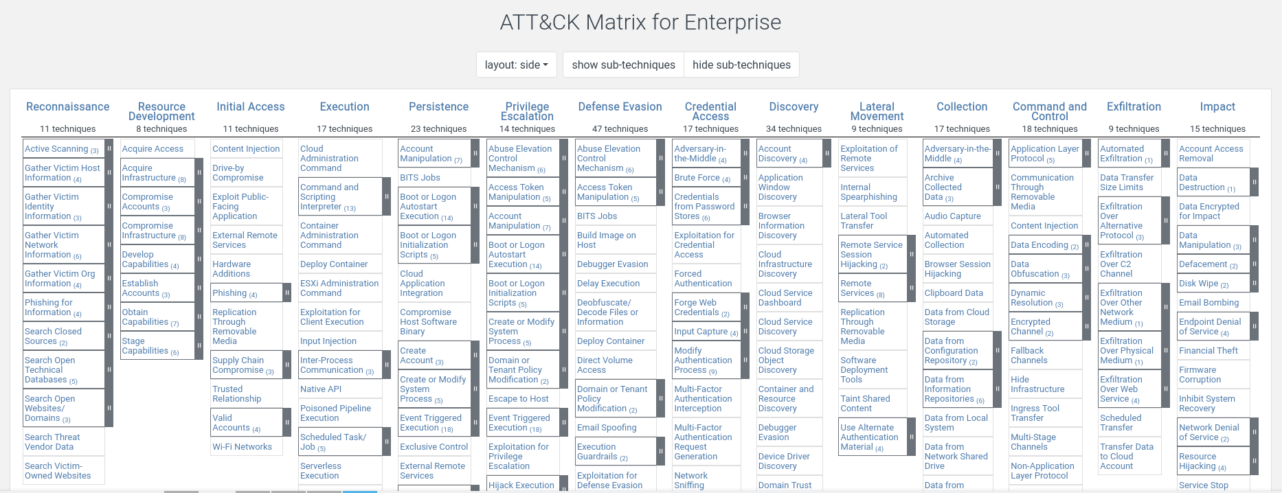
You can find this matrix here. The idea is that from left to right you get the logical flow of an attack from the attacker’s perspective - from reconnaissance, all the way to data exfiltration and impact on your organization. In MITRE’s naming, each step is a tactic, and each tactic contains the techniques an attacker can use.
Example: once the first host is compromised, an attacker often wants to survive a reboot - that’s what we call persistence. Technique T1053: Scheduled Task/Job documents that an attacker can set up scheduled tasks to ensure their malware will be relaunched later despite a reboot.
From a network standpoint, most of these steps are clearly visible if you have the right capture points. The only steps that could really escape our view are:
- persistence
- privilege escalation
- defense evasion
Since these steps are local by nature, it’s rarely possible to observe them on the network. Note that depending on our observation point we could miss other steps as well. For example, if we only observe an egress point to the internet, it’s impossible to see lateral movement between machines.
The kill chain steps (the attack chain) that are most detectable from the network are mainly:
- command and control: because malware must communicate with its server
- lateral movement: pretty noticeable, because connections from one machine to another on certain ports can be unexpected
- data exfiltration: if done poorly, a sudden increase in data volume can be noticeable
For an example of lateral movement visible from the network, I invite you to read my article on the dce-rpc backdoor.
Limits of network analysis
We’ve already seen some limits of network analysis above, but other issues still remain - like encryption. A lot of communications are encrypted now and rely on TLS, preventing us from having a clear view of the payloads. We can still see who talks to whom without seeing the content; and from that point of view we’re limited to deciding whether something is simply suspicious or not. That’s one of the reasons you need to correlate network observation with host analysis as part of incident response.
NAT often causes headaches for the analyst. With the IPv4 address shortage, an outbound connection often goes like this:
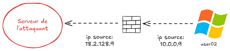
So, if we observe the connection from outside the firewall, we’ll struggle to determine who the source machine is, because their IP addresses are all replaced with the firewall’s IP. It’s not impossible, but it’s more complicated - which is why we generally try to observe traffic from inside the firewall.
Setup and data loading
Now that we’ve quickly introduced why network forensics matters, let’s discover and exploit our data!
Dataset
For this first analysis we’ll use a dataset provided by dfir-madness. It’s a pcap, meaning a file that records all data exchanged on a network.
The author of that site provides a few datasets to practice forensics - the art of making data speak so you can find traces of past events.
As you understood above, a serious cyber problem appeared in the company storing the Szechuan sauce recipe. So we’ll try to answer the question: was the sauce secret stolen?
Tooling
In forensics, once you have raw data, two steps remain. Parsing (extracting data in a reproducible and intelligible way), then indexing it into a tool that enables querying.
In this article, we’ll keep it simple with two well-known open source tools: Zeek and Python.
Why not Wireshark? Wireshark is perfect to analyze a small capture or develop detection rules, but it doesn’t scale at all. Also, it’s not reproducible and it’s hard to automate.
Zeek
Zeek is a wonderful open source tool that parses (i.e., extracts useful data) from a network capture. If you talk to it nicely, it can extract pretty much any protocol in different formats - including JSON.
Zeek can also be extended with plugins, as well as its own scripting language.
Python
To avoid the pain of building a SIEM, we’ll use something much more versatile: Python. Thanks to the pandas library, Python is perfect to load tabular data, process it, and query it - which is exactly what we need for forensics.
We’ll do our analysis in JupyterLab, where we’ll write as we go. This article doesn’t present JupyterLab itself, but rather a condensed version.

Installing dependencies
For Zeek, we’ll install it via Docker to make installation easier. I invite you to install Docker by following your distribution’s documentation.
Then we can download the available Dockerfile and build the image:
mkdir zeek && cd zeek
wget https://raw.githubusercontent.com/theophane-droid/blog_content/refs/heads/main/network_investigation/docker/Dockerfile
docker build -t custom_zeek . # build the zeek image
And for Python, we’ll create a dedicated virtual environment and install our dependencies inside it:
python3 -m venv venv
source venv/bin/activate
pip install jupyterlab pandas
Dissecting pcaps
To begin our analysis, we’ll download the Zeek script available here: profile.zeek. That Zeek script describes the different protocols we’ll dissect, which configurations we load, and other automations.
If we look at the beginning of the script:
@load base/protocols/conn
@load base/protocols/dns
@load base/protocols/http
@load base/protocols/ssl
@load base/protocols/smtp
@load base/protocols/ftp
@load base/protocols/ssh
Here we load several Zeek scripts that let us analyze DNS, HTTP, SMTP, FTP, TLS and SSH.
For each of these protocols, Zeek will create a .log file containing parsed sessions in an intelligible form.
As for conn, Zeek will simply extract all connections into a file named conn.log.
Let’s proceed with extracting the data:
docker run --rm --name zeek -v .:/analysis -w /analysis custom_zeek \
    zeek -r /analysis/sample.pcap /analysis/profile.zeek -e 'redef LogAscii::use_json=T;'
A quick explanation of the command above is needed. First the beginning: docker run --rm --name zeek -v .:/analysis -w /analysis custom_zeek.
We start a container with the Zeek image we built earlier, specifying that we mount the current directory into /analysis with -v.
We also specify that we’ll work in the /analysis directory inside the container with -w.
The second part: zeek -r /analysis/sample.pcap /analysis/profile.zeek -e 'redef LogAscii::use_json=T;' runs Zeek in the container and points it at our profile.
We run Zeek on a file named sample.pcap - the pcap we’re analyzing - and we specify via -e that we want JSON output.
The analysis shouldn’t take more than a minute or two, and once it’s done we get the following files:
~/project/blog_content/network_investigation> ls
╭────┬───────────────────┬──────┬──────────┬────────────────╮
│  # │       name        │ type │   size   │    modified    │
├────┼───────────────────┼──────┼──────────┼────────────────┤
│  0 │ capture_loss.log  │ file │   2.3 kB │ 2 minutes ago  │
│  1 │ conn.log          │ file │  13.3 MB │ 2 minutes ago  │
│  2 │ dce_rpc.log       │ file │  49.3 kB │ 2 minutes ago  │
│  3 │ dns.log           │ file │ 867.1 kB │ 2 minutes ago  │
│  4 │ files.log         │ file │ 339.0 kB │ 2 minutes ago  │
│  5 │ http.log          │ file │ 124.1 kB │ 2 minutes ago  │
│  6 │ kerberos.log      │ file │  20.0 kB │ 2 minutes ago  │
│  7 │ ldap.log          │ file │  38.1 kB │ 2 minutes ago  │
│  8 │ ldap_search.log   │ file │  71.2 kB │ 2 minutes ago  │
│  9 │ notice.log        │ file │  68.1 kB │ 2 minutes ago  │
│ 10 │ ocsp.log          │ file │ 246.7 kB │ 2 minutes ago  │
│ 11 │ packet_filter.log │ file │     90 B │ 2 minutes ago  │
│ 12 │ pe.log            │ file │    792 B │ 2 minutes ago  │
│ 13 │ profile.zeek      │ file │    499 B │ 44 minutes ago │
│ 14 │ rdp.log           │ file │  23.2 kB │ 2 minutes ago  │
│ 15 │ sample.pcap       │ file │ 197.5 MB │ 5 years ago    │
│ 16 │ smb_files.log     │ file │  14.0 kB │ 2 minutes ago  │
│ 17 │ smb_mapping.log   │ file │   5.0 kB │ 2 minutes ago  │
│ 18 │ ssl.log           │ file │   6.4 MB │ 2 minutes ago  │
│ 19 │ weird.log         │ file │   6.1 kB │ 2 minutes ago  │
│ 20 │ x509.log          │ file │ 145.8 kB │ 2 minutes ago  │
╰────┴───────────────────┴──────┴──────────┴────────────────╯
So we do have one .log file per protocol recognized by Zeek. As explained above, conn.log describes all the connections
that occurred in the pcap, and those same connections will be described again in the appropriate protocol .log.
Let’s look at the first line of conn.log using jq (a very handy tool for opening JSON):
~/project/blog_content/network_investigation> head -n 1 conn.log | jq
{
  "ts": 1600466289.552099,
  "uid": "CY4WhX1MsAdfYVW5rc",
  "id.orig_h": "fe80::2dcf:e660:be73:d220",
  "id.orig_p": 54064,
  "id.resp_h": "ff02::1:3",
  "id.resp_p": 5355,
  "proto": "udp",
  "service": "dns",
  "duration": 0.4179189205169678,
  "orig_bytes": 60,
  "resp_bytes": 0,
  "conn_state": "S0",
  "local_orig": true,
  "local_resp": false,
  "missed_bytes": 0,
  "history": "D",
  "orig_pkts": 2,
  "orig_ip_bytes": 156,
  "resp_pkts": 0,
  "resp_ip_bytes": 0,
  "ip_proto": 17,
  "ja4l": "",
  "ja4ls": "",
  "ja4t": "",
  "ja4ts": ""
}
Zeek describes here the connection between a source IP id.orig_h and a destination IP id.resp_h.
Notice how Zeek gives us varied information about source/destination ports, connection duration, bytes exchanged in both directions, etc.
If for example we look at the first entry of dns.log with jq:
~/project/blog_content/network_investigation> head -n 1 dns.log | jq
{
  "ts": 1600466289.552099,
  "uid": "CY4WhX1MsAdfYVW5rc",
  "id.orig_h": "fe80::2dcf:e660:be73:d220",
  "id.orig_p": 54064,
  "id.resp_h": "ff02::1:3",
  "id.resp_p": 5355,
  "proto": "udp",
  "trans_id": 26344,
  "query": "citadel-dc01",
  "qclass": 1,
  "qclass_name": "C_INTERNET",
  "qtype": 255,
  "qtype_name": "*",
  "AA": false,
  "TC": false,
  "RD": false,
  "RA": false,
  "Z": 0,
  "rejected": false,
  "opcode": 0,
  "opcode_name": "query"
}
Here dns.log describes the same session as the previous conn.log, which we can see via the uid field being strictly identical.
Compared to conn, dns.log gives us additional DNS-specific information: query type, query name, response, whether it succeeded, etc.
We can also mention weird.log, which lists anomalies spotted by Zeek. That can be an interesting starting point for analysis.
Each standard Zeek log type is described here in the documentation.
Loading and exploring the data
Once our pcap has been processed by Zeek, we can launch JupyterLab from our terminal:
jupyter lab
Make sure to copy the URL returned by the command, including the token that lets you log in. In Jupyter, we can start by creating a code cell to import our dependencies and configure pandas:
import os
import pandas as pd

pd.set_option("display.max_rows", 50)
pd.set_option("display.max_columns", None)
pd.set_option("display.max_colwidth", None)
pd.set_option("display.width", None)
Then load all our datasets and convert all timestamps into a readable format (careful: we’re in UTC):
datasets = {}
for file in os.listdir('.'):
    if file.endswith('.log'):
        name = file.split('.')[0]
        datasets[name] = pd.read_json(file, lines=True)
        datasets[name]["dt_utc"] = pd.to_datetime(datasets[name]["ts"], unit="s", utc=True)
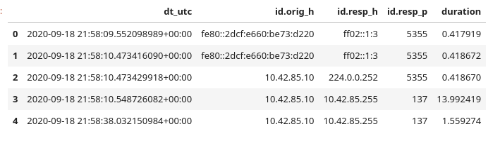
Finally we can display the first connections like this:
conn = datasets['conn']
conn[['dt_utc', 'id.orig_h', 'id.resp_h', 'id.resp_p', 'duration']].head()
To wrap up, here are a few examples of using pandas to analyze our data:
# 1. Top 5 most active destinations (by number of connections)
conn['id.resp_h'].value_counts().head(5)

# 2. Identify suspicious data transfers (> 1 MB)
conn[conn['resp_bytes'] > 1000000][['id.orig_h', 'id.resp_h', 'service', 'resp_bytes']]

# 3. List all resolved domains (DNS) to spot beaconing
datasets['dns']['query'].unique()
Conclusion
Done! We’re now ready to start the analysis in JupyterLab! As we’ll see, one of the big advantages of the tool is being able to alternate code cells and markdown cells, so we can comment our analysis at every step.
To summarize, in this article we understood the basics of network investigation, and we saw how to extract our data with Zeek and load it into JupyterLab.
In the next article we’ll take a closer look at our data and find the malicious actions that could have led to the theft of the Szechuan sauce. On the menu: initial access, lateral movement, and exfiltration - see you in the next article for the investigation itself. See you soon!